What This Investigation Covers
We evaluate two models on 50 binary test cases, and the bar chart says the wrong model wins. This investigation builds from that synthetic example to a full statistical workflow: computing confidence intervals on the pairwise difference, tightening estimates with multiple runs, and validating the approach on a real sentiment analysis eval.
What you’ll learn
Why the apparent winner can be wrong: An example where the model with the higher true rate loses in the sample, building intuition for why raw means at N=50 routinely mislead.
How to compute a CI on the pairwise difference: Using estats.compare_models() for paired binary data, and reading the output interval to decide whether the gap is real.
Why multiple runs improve your estimates: Adding 10 runs per input activates the nested bootstrap, which accounts for both input-level and run-level variance and produces more honest uncertainty bounds.
How to work with a real eval CSV: Pivoting a tidy multi-run CSV from a sentiment analysis eval into the format compare_models expects: a complete data-loading walkthrough.
Looking for quick usage examples? Check out the Example Usage page.
Suppose we evaluate two models on the same prompt template with 50 inputs: a paired design where both models see every item and receive a binary score: 1 if the response passes, 0 if it fails.
Why paired? Pairing is essential: comparing two models on different inputs conflates model quality with input difficulty. Always run both models on the same test set.
We'll use synthetic data here, but everything carries over to real eval results.
import numpy as np

rng = np.random.default_rng(42)
N = 50

# Synthetic binary scores: true pass rates are 70% (A) and 60% (B)
scores_a = rng.binomial(1, 0.70, N).astype(float)
scores_b = rng.binomial(1, 0.65, N).astype(float)

mean_a = scores_a.mean()
mean_b = scores_b.mean()
obs_diff = mean_a - mean_b

print(f"Model A:  {mean_a:.1%}  ({int(scores_a.sum())}/{N} passed)")
print(f"Model B:  {mean_b:.1%}  ({int(scores_b.sum())}/{N} passed)")
print(f"Gap:     {obs_diff:+.1%}")
Notice anything wrong?
We rigged Model B to be worse — yet it came out ahead (72% vs 64%).
This isn't a bug. LLM evaluation is random sampling: each prompt is a coin flip, and with only 50 flips per model, results can easily invert. The same thing happens with real models on real benchmarks.
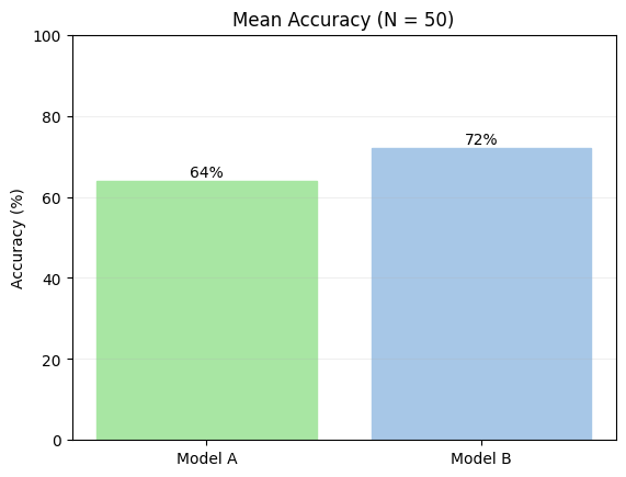
Most eval platforms stop here — they show you this bar chart, and you conclude Model B is better. With N=50, that conclusion is unreliable. A bare mean has no error bars, no sense of how much it could shift with a different sample. We need a confidence interval.
Computing a Confidence Interval
A confidence interval (CI) quantifies uncertainty around an estimate. A 95% CI means: if you repeated this experiment many times, roughly 95% of those intervals would contain the true value. When the CI for a difference includes zero, the data cannot rule out that the true gap is zero.
evalstats's compare_models() returns a CI on each model's mean and on the gap between them.
We pass
method="auto", which inspects the data type and study design to select an appropriate statistical method automatically. For more info on these defaults and their rationale, see Which Method.
import evalstats as estats

# Set the global alpha for CIs to 0.05 for this example - this creates "95%" confidence intervals (1-alpha).
# It's good practice to declare this explicitly in your code, before running any tests.
estats.set_alpha_ci(0.05)

# Compare the two models (the 'auto' method will choose appropriate methods based on the data)
report = estats.compare_models(
    {"Model A": scores_a, "Model B": scores_b},
    method="auto",
    rng=np.random.default_rng(0),
)

report.print_ci_table()
print()
report.print_pair("Model A", "Model B")
Reading the Output
Model B came out ahead in this sample by the mean gap of -8.0%. But this is only an estimate from 50 samples, it doesn't tell you how reliable that gap is.
The 95% CI of [-26.0%, +10.0%] is what matters here: the true difference between models could plausibly be anywhere in that range. The interval straddles zero (│), so the data can't rule out that there's no real difference.
Since we used synthetic data, we know the true means. Notice that the true difference,
+5.0%, is included in the 95% CI range—stats is doing its job.
The 95% CI is keeping us honest. With N=50 and a small true gap, there's simply not enough signal yet. The goal is to collect more inputs and watch the interval narrow. A result like this would let you draw a firmer conclusion:
Model B (<0) ··───●───·· | (>0) Model A
Until we see something like that, the right call is to withhold judgment and keep collecting data.
We have two options for that—either we expand our test set, or we add runs to combat the potential randomness in model performance. Let's try the latter.
Method note:
bayes binarymeansevalstatsdetected binary data and used Bower et al.'s Bayesian pairwise method for the CI. For why it chose this method, see Which method. To use a different method, pass e.g.method="newcombe".
Effect sizes and p-values
Before we continue, you might've noticed two other parts of this output—an effect size, and a p-value. Let's explain these.
An effect size answers a different question than a CI or p-value. The CI tells you how uncertain your estimate is; the effect size tells you how large the difference is, on a standardized scale that makes it easier to compare across experiments. In our output, the rank-biserial effect size -0.200 for A - B is considered small-to-moderate (see note below), which is a modest directional trend towards B.
A p-value is the probability of observing results at least as extreme as your data, assuming there's no difference between the things you're comparing (i.e., that the "null hypothesis" is true—or here, that Models A and B produce the same outputs). A small p-value (typically below 0.05) suggests that our results are unlikely to occur by chance. Although evalstats can report p-values, the p-value provides redundant information to confidence intervals—if a CI doesn't straddle zero, it's essentially the same as a $p < 0.05$ (or your chosen $\alpha$ of choice).
evalstatsreports rank-biserial correlation (r_rb) as its effect size. You might be more familiar with Cohen's d, the classic effect size for comparing two means. Cohen's d assumes scores are continuous and approximately normally distributed. LLM outputs don't necessarily follow normality assumptions: scores are often binary (pass/fail), bounded (e.g. 1–5 Likert scales), or skewed. Rank-biserial correlation sidesteps this by working purely on the ranks of paired differences, with no distributional assumptions. Its value ranges from −1 to +1:
| Rank-biserial Effect Size | Interpretation |
|---|---|
| ±0.1 | Small effect — likely negligible in practice |
| ±0.3 | Moderate effect — worth investigating further |
| ±0.5 | Large effect — practically meaningful |
For p-values here,
evalstatsreported the Wilcoxon signed-rank test, a non-paremetric test and chosen for two reasons: 1) it is widely used in this scenario, and 2) it was the most performant in our simulations of evals-like data (best on-target coverage across distributions).
Multiple Runs Reduce Noise
LLMs are stochastic: the same input on a different call can yield a different score. Running each input once means some of your variance comes from model randomness, not true performance differences.
Adding multiple runs per input lets us separate that noise from the signal. With multiple runs, the data is a list of inputs, each holding a list of per-run scores, for instance:
model_a_runs = [
    [1.0, 1.0, 0.0, 1.0, 0.0],  # input 0: scores across 5 runs
    [0.0, 1.0, 1.0, 0.0, 1.0],  # input 1
    ...                         # 50 inputs total, with 5 runs each
]
We can pass these nested lists directly to compare_models() and it'll detect the structure automatically. We'll use N_RUNS = 10 and synthetic data again, just to show the concept:
import random
random.seed(43)

N_INPUTS = 50
N_RUNS = 10

# Same true pass rates as before: 70% (A), 65% (B)
model_a_runs = [
    [1.0 if random.random() < 0.70 else 0.0 for _ in range(N_RUNS)]
    for _ in range(N_INPUTS)
]
model_b_runs = [
    [1.0 if random.random() < 0.65 else 0.0 for _ in range(N_RUNS)]
    for _ in range(N_INPUTS)
]

report_multirun = estats.compare_models(
    {"Model A": model_a_runs, "Model B": model_b_runs},
    method="auto",
    rng=np.random.default_rng(1),
)

pair_multirun = report_multirun.pairwise.get("Model A", "Model B")
pair_multirun.summary()
Now Model A comes out on top, but still not significantly. The 95% CI [-6.7%, +30.7%] still straddles zero. Ten runs per input was enough to tighten the CI, but the noise and closeness of the underlying means still leaves us unsure.
Real-World Example
The synthetic setup builds intuition, but in practice you load results from real model runs. Below we use a sentiment analysis eval from examples/compare_models_multirun.py, which outputs a CSV with one row per model × input × run:
| model_name | template_label | input_idx | run_idx | accuracy |
|---|---|---|---|---|
| gpt-4.1-nano | Minimal | 0 | 0 | 1.0 |
| gpt-4.1-nano | Minimal | 0 | 1 | 1.0 |
| mistralai/ministral-8b-2512 | Minimal | 0 | 0 | 0.0 |
| ... | ... | ... | ... | ... |
The eval covers two models, several prompt templates, 27 inputs, and 3 runs each. We'll focus on the Minimal template.
import pandas as pd
from pathlib import Path

csv_path = "basic_sentiment_eval_2models.csv"
df = pd.read_csv(csv_path)

# Filter to the template we want
minimal = df[df["template_label"] == "Minimal"].copy()

# Pivot to (input_idx, run_idx) × model_name
pivot_df = minimal.pivot(
    index=["input_idx", "run_idx"],
    columns="model_name",
    values="accuracy"
).dropna()

# Reshape to {model: [[input0_runs], [input1_runs], ...]}
scores_by_model = {
    model: pivot_df[model].groupby("input_idx").apply(list).tolist()
    for model in pivot_df.columns
}

# Run the comparison
report = estats.compare_models(
    scores_by_model,
    method="auto",
    rng=np.random.default_rng(7),
)

pair = report.pairwise.get("gpt-4.1-nano", "mistralai/ministral-8b-2512")
pair.summary()
With 27 inputs and 3 runs, the CI [-3.8%, +18.6%] still spans zero. We're leaning toward gpt-4.1-nano, but the data can't rule out chance. The path forward: expand the test set (more inputs), increase the number of runs, or both. Watch whether the CI narrows and moves clear of zero as you do.
Next Investigation
Check out Finding Your Best Prompt, which introduces a few new concepts—pairwise comparisons and multiple comparisons correction to control the family-wise error rate (FWER). If you're still wrapping your head around what CIs are, check out the interactive widget below.
Interactive Visualizer
The examples above each showed a single CI from a single experiment. To build intuition for why CIs vary and what "95% confidence" actually means, run the visualization below.
Each click simulates a fresh eval — drawing a new sample, computing a CI, and stacking it in the lower panel. Green intervals capture the true effect; red ones miss. Over many runs, roughly 95% should be green (for α = 0.05) — that's exactly what "95% confidence" guarantees.
- Top panel: sampled scores and per-model means for one eval run
- Bottom panel: accumulated CIs across all runs
Try increasing N or reducing the true effect to see how CI width changes.