Recommendations and Defaults
We have run the most comprehensive simulation study to date on confidence interval methods for LLM eval data, and with few exceptions,
we have validated these results on real eval data as well. Based on this research, we recommend the following methods for
calculating confidence intervals in LLM eval contexts. We also performed a smaller simulation study on p-value methods, and report recommendations as well.
These recommendations are implemented as the
method="auto" defaults in evalstats,
which adapt to data type and sample size based on which methods performed best in our simulations.
Note that the contents of this section are subject to change as we gather more evidence for different situations.
Recommended Confidence Intervals Methods (By Data Type and Type of Comparison)
Point estimates
Pairwise comparisons
Point estimates
Pairwise comparisons
tango_multirun_mmnt is the fastest and best-calibrated multi-run binary pairwise method (0.957),
validated in both our synthetic and real-data simulations.
As far as we know, this is a novel multi-run extension of the Tango score interval which was proposed by GPT-5.
Recommended p-value methods by analysis type
| Task | Data Type | Recommended Method | Notes |
|---|---|---|---|
| Pairwise test (A vs B) | Any paired eval scores | Wilcoxon Signed Ranks | Slightly conservative, consistent across data types and sample sizes, and no Type I inflation above the alpha in our simulation. |
| Pairwise test (A vs B), but in a safety-critical setting | Any paired eval scores | Sign Test | More conservative than Wilcoxon; useful when false positives are very costly. |
| Multiple pairwise tests (k variants) | Any | Benjamini-Hochberg (fdr_bh) |
Default correction in evalstats; controls expected false discovery rate with better power than stricter family-wise procedures. |
Do not rely on NHST alone for eval decisions. If you report p-values, report them alongside effect sizes and confidence intervals. Prefer effect sizes and CIs as primary evidence, and treat p-values as secondary.
Sample Size Guidance
N < 15: Do not report statistics. The CI width will be so large as to be meaningless, and the sample is extremely unlikely to be representative.
15 ≤ N < 30: Report statistics with a prominent warning. Results should be treated as exploratory only.
N ≥ 30: CIs and point estimates of true performance begin to become more reliable.
Simulation Study: Which CI method should I use in X situation?
We ran comprehensive simulation studies over eval-like distributions to compare methods for calculating CIs head-to-head— to the best of our knowledge, the most comprehensive test of CI methods ever conducted for small-sample AI evals data. We compared almost all known CI methods (and even a few ones invented with the help of AI) to see which ones are best for different data types, sample sizes, and estimands. We also measured the computational cost of each method, since some of the more complex methods can be very expensive to run at scale. Finally, we validated the results on real eval data by subsampling from real benchmark outputs, to double-check how well the simulation findings hold up in practice.
How to measure CI "performance"?
A confidence interval (CI) is only useful if it's trustworthy, tight, and fast to compute. We measure CI quality along three dimensions:
- Coverage: If you ask a method to build a 95% CI, it should actually contain the true value 95% of the time across many repeated experiments. A method with under-coverage (say, 88%) gives intervals that are too narrow and misleadingly confident. A method with over-coverage (say, 99%) is overly conservative—it works, but it may be too cautious. We target nominal coverage of 95% for all simulations.
- Width: Once a method achieves good coverage, narrower intervals are better. Width measures how "confident" the CI is: all else equal, the method that produces the tightest interval while still hitting 95% coverage wins.
- Cost: how long the method takes to run. Simple analytic formulas (like the Wilson interval for binary scores) compute in microseconds. Resampling methods like the bootstrap require thousands of resampled datasets and can take seconds or more, especially as the sample size increases. Cost matters when you're running evaluations over many models, prompts, or benchmarks simultaneously.
In practice, coverage comes first—a cheap, narrow interval that's wrong 20% of the time is useless. Among methods that achieve adequate coverage, we prefer narrower intervals, and among those, faster ones.
Methodology
We rigged realistic distributions, randomly sampled from them, then measured how close each CI
method gets to the true value across repeated trials. Two estimands were tested: single-sample CIs
(does the interval contain the true mean?) and pairwise difference CIs (does the interval contain
the true difference?). Sample sizes: N = 10, 15, 20, 30, 40, 50, 60, 70, 80, 90, 100. Bootstrap and Bayesian draws: 10,000.
Monte-Carlo trials: 2,000 per condition. We also validated on real LLM eval data by subsampling from 1)
OpenEvals outputs across 15 unique model × benchmark pairs, for the single-run case, and 2)
outputs of six models across nine benchmarks run 5 times per benchmark, for the multi-run case. Simulations are implemented in
simulations/ folder in the project repository.
Distributions Tested
Across our synthetic simulations, we tested the following four data types (our simulations using real data test only the first two, binary and continuous):
- Binary scores ({0, 1}): Bernoulli with p ∈ {0.02, 0.05, 0.1, 0.3, 0.5, 0.7, 0.9, 0.95, 0.98} (9 scenarios)
- Continuous scores (0–1 floats): Beta families — uniform Beta(1,1), U-shaped Beta(0.5,0.5), right-skewed Beta(2,8), left-skewed Beta(8,2), moderate-skew Beta(2,5), extreme-right Beta(0.35,6), extreme-left Beta(6,0.35), near-boundaries Beta(0.3,0.3), near-center Beta(6,6), mixture of Beta(0.5,4) and Beta(5.5,1.2); plus a logit-normal (μ=−0.35, σ=1.35), zero-inflated (70% spike at 0, Beta(2,4) body), and one-inflated (70% spike at 1, Beta(4,2) body) (13 scenarios)
- Likert scores (integers 1–5): latent-normal model rounded and clipped to 1–5, covering uniform (high variance), skewed-low, skewed-high, bimodal (peaks at extremes), center-peaked, near-floor, near-ceiling, polarized, and flat-middle (9 scenarios)
- Grades (0–100 floats): clipped-normal scenarios — symmetric N(50,20), high-scoring N(75,15), low-scoring N(35,20), ceiling-heavy N(88,10), floor-heavy N(12,10), very-high N(92,7), very-low N(8,7), high-variance N(50,34); plus a 3-component truncated-normal mixture, a heavy-tailed t(df=3) distribution, a zero-spiked (40% spike at 0, N(45,20) body), and a hundred-spiked (40% spike at 100, N(65,18) body) (12 scenarios)
Single-Sample Coverage (target: 0.95)
The following image and table presents the results of the Monte Carlo simulation. The table breaks down the final average coverage rates at each sample size, with notes on performance. (Coverage rate = fraction of trials where the CI contains the true population mean. Higher is better; under-coverage means the method is over-confident.)
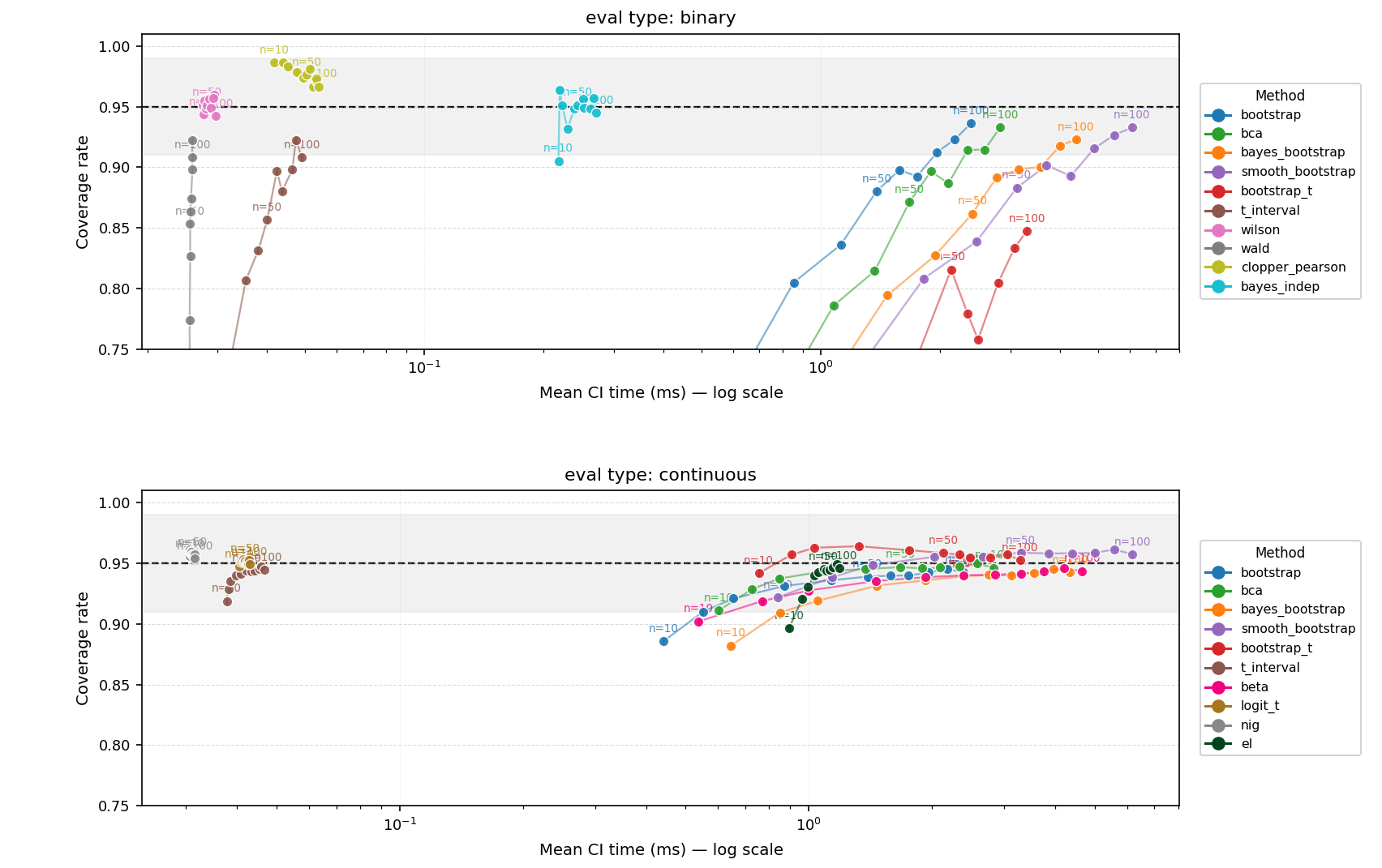
| Method | Coverage | Time (ms) | Width | Dev | Data types |
|---|---|---|---|---|---|
| Percentile bootstrap | 0.911▼ | 1.346±0.001 | 3.3176 | -0.039 | Any |
| BCa | 0.913▼ | 1.635±0.001 | 3.3392 | -0.037 | Any |
| Bayes bootstrap | 0.908▼ | 2.376±0.001 | 3.2552 | -0.042 | Any |
| Smooth bootstrap (Gaussian KDE) | 0.929 | 3.273±0.002 | 3.7557 | -0.021 | Any |
| Bootstrap-t | 0.910▼ | 1.981±0.001 | 3.7062 | -0.040 | Numeric (continuous/discrete) |
| Student's t-interval | 0.918 | 0.042±0.000 | 3.6109 | -0.032 | Numeric (continuous/discrete) |
| Wilson score interval ★ | 0.951 | 0.029±0.000 | 0.2033 | +0.001 | Binary |
| Wald interval | 0.806▼ | 0.026±0.000 | 0.1716 | -0.144 | Binary |
| Clopper-Pearson | 0.977 | 0.049±0.000 | 0.2236 | +0.027 | Binary |
| Bayesian independent samples | 0.946 | 0.243±0.000 | 0.2037 | -0.004 | Binary |
| Beta interval | 0.934 | 2.442±0.003 | 0.1361 | -0.016 | Continuous [0, 1] (non-binary) |
| Logit-t ★ | 0.951 | 0.042±0.000 | 0.1443 | +0.001 | Continuous [0, 1] |
| Normal-Inverse-Gamma (NIG) ★ | 0.958 | 0.031±0.000 | 0.1430 | +0.008 | Continuous [0, 1] |
| Empirical likelihood (EL) | 0.937 | 1.069±0.001 | 0.1327 | -0.013 | Numeric (continuous/discrete) |
Coverage target is 0.95. ▼ marks under-target coverage. ★ marks preferred methods. Methods with a scope note (binary only / continuous [0, 1] only) are not applied to other data types; their numbers are therefore not directly comparable to general-purpose methods. Bootstrap-family methods are averaged across all data types. MCSE values are negligible (around ~0.005 or lower), so they are omitted from this display.
Single-Sample Coverage on Real LLM Eval Data (target: 0.95)
To complement the synthetic simulation, we also evaluated CI methods on real LLM evaluation data by randomly drawing samples from evaluation score outputs in the OpenEvals dataset, across 15 unique model × benchmark pairs, for variety. Coverage was measured by repeatedly subsampling from each benchmark's full score distribution and checking whether the CI contained the true (full-population) mean. This tests how methods behave on actual eval data shapes, which may differ from the idealized distributions in the synthetic study.
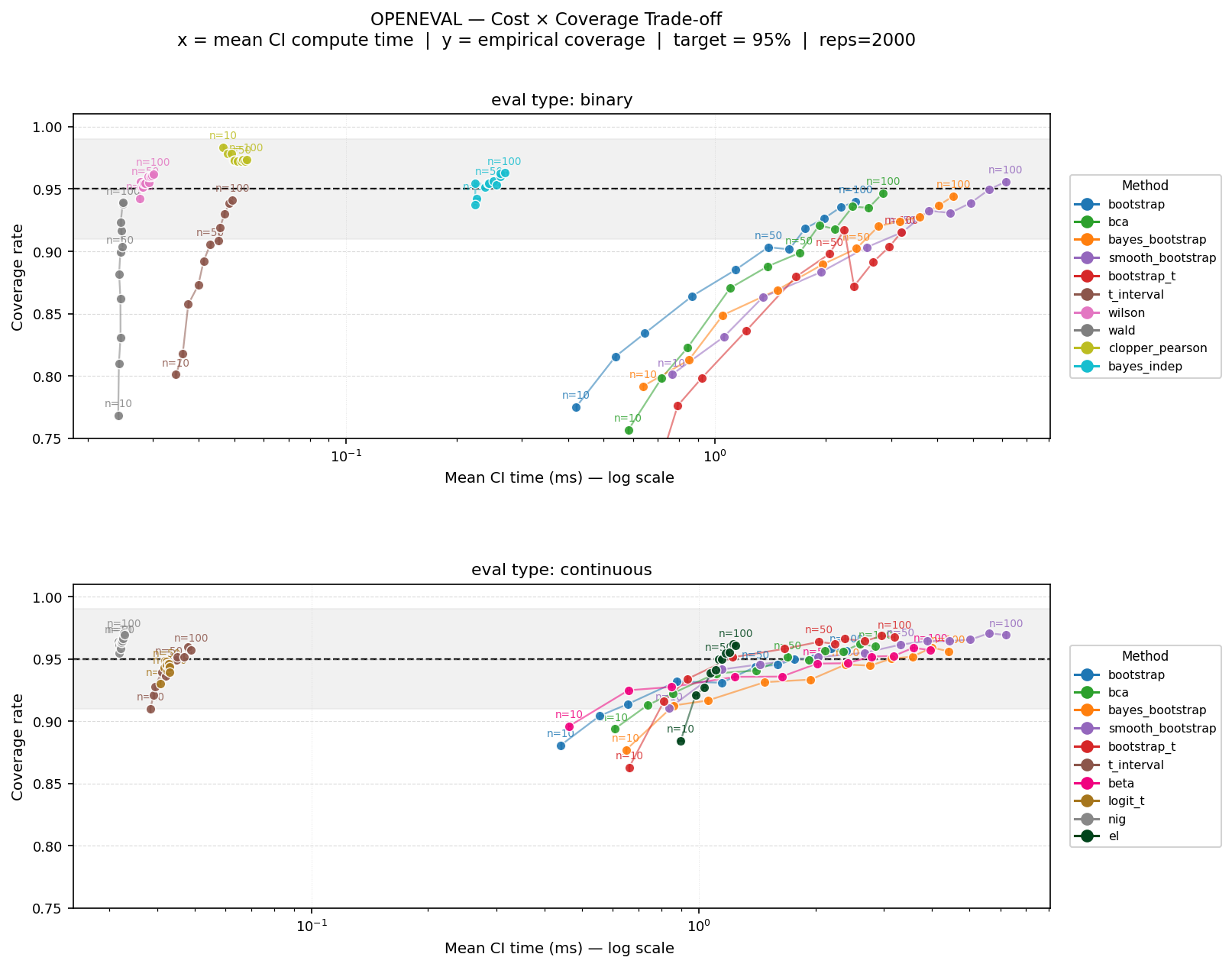
| Method | Coverage | Time (ms) | Width | Dev | Data types |
|---|---|---|---|---|---|
| Percentile bootstrap | 0.899▼ | 1.359±0.001 | 0.2082 | -0.051 | Any |
| BCa | 0.901▼ | 1.656±0.001 | 0.2184 | -0.049 | Any |
| Bayes bootstrap | 0.903▼ | 2.395±0.002 | 0.2042 | -0.047 | Any |
| Smooth bootstrap (Gaussian KDE) | 0.918 | 3.269±0.003 | 0.2381 | -0.032 | Any |
| Bootstrap-t | 0.884▼ | 1.887±0.001 | 0.2250 | -0.066 | Numeric (continuous/discrete) |
| Student's t-interval | 0.907▼ | 0.043±0.000 | 0.2293 | -0.043 | Numeric (continuous/discrete) |
| Wilson score interval ★ | 0.955 | 0.029±0.000 | 0.2521 | +0.005 | Binary |
| Wald interval | 0.879▼ | 0.025±0.000 | 0.2476 | -0.071 | Binary |
| Clopper-Pearson | 0.975 | 0.051±0.000 | 0.2793 | +0.025 | Binary |
| Bayesian independent samples | 0.953 | 0.246±0.001 | 0.2531 | +0.003 | Binary |
| Beta interval | 0.939 | 2.073±0.004 | 0.1334 | -0.011 | Continuous [0, 1] (non-binary) |
| Logit-t | 0.943 | 0.042±0.000 | 0.1434 | -0.007 | Continuous [0, 1] |
| Normal-Inverse-Gamma (NIG) ★ | 0.964 | 0.032±0.000 | 0.1423 | +0.014 | Continuous [0, 1] |
| Empirical likelihood (EL) | 0.940 | 1.109±0.002 | 0.1307 | -0.010 | Numeric (continuous/discrete) |
Coverage target is 0.95. ▼ marks under-target coverage. ★ marks preferred methods. Methods with a scope note (binary only / continuous [0, 1] only) are not applied to other data types. Results are averaged across 15 model × benchmark pairs and all sample sizes.
Pairwise Comparison Coverage (target: 0.95)
For paired comparisons, coverage measures whether the CI on the difference contains the true difference. This is the more practically important statistic for comparing two prompts or models.
Pairwise scenarios are parameterised by two factors that are swept jointly: the intraclass correlation (ICC), which captures how much variance is attributable to the input (prompt/example) rather than the model, and the standardised effect size (Cohen's d), which sets the true difference between the two candidates. The official test sweeps ICC ∈ {0.05, 0.15, 0.30, 0.50} and d ∈ {0.0, 0.2, 0.4} (the d = 0 condition measures Type I error rate; the non-null conditions measure coverage under a real effect). ICC is implemented differently per data type: a Beta-hierarchical model for binary scores, a Gaussian-noise perturbation of a Beta base for continuous scores, and a latent-normal model for Likert and grades. All pairwise scenarios also use the full expanded scenario suite, so the distributions tested are the same rich set described above.
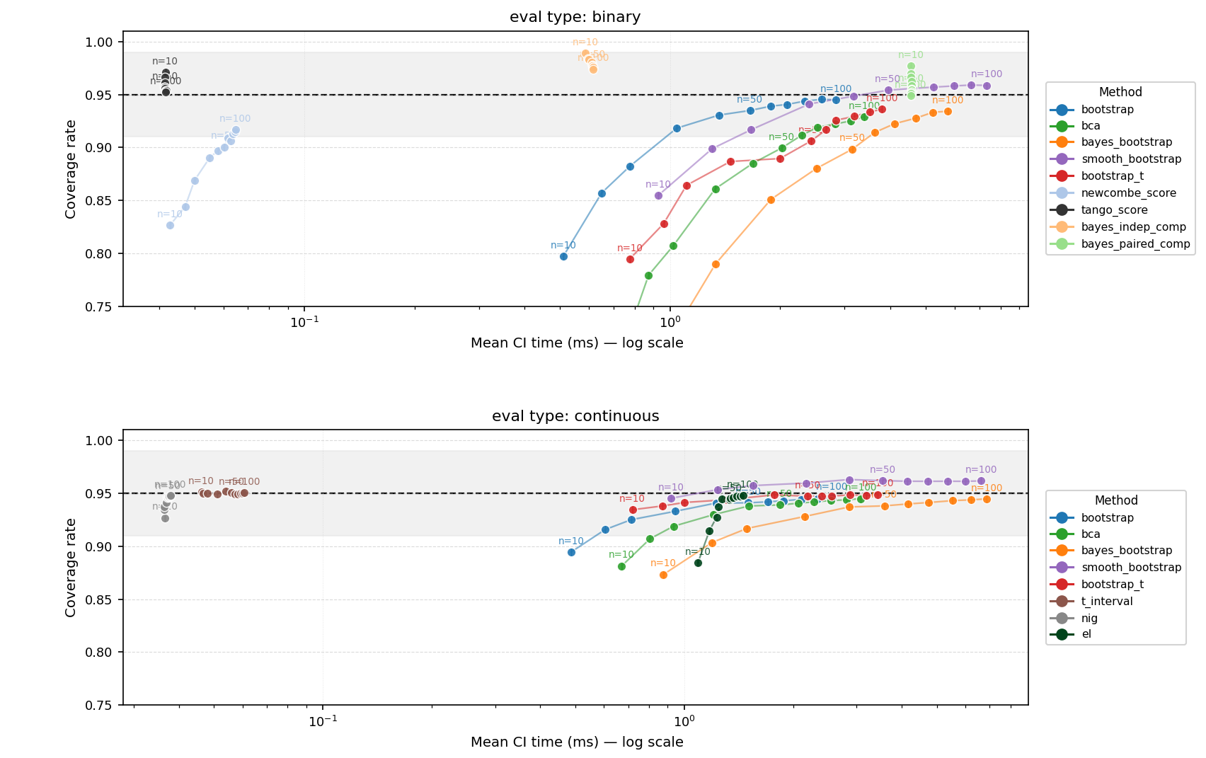
| Method | Coverage | Time (ms) | Width | Dev | Data types |
|---|---|---|---|---|---|
| Percentile bootstrap | 0.922 | 1.458±0.000 | 2.7531 | -0.028 | Any paired |
| BCa | 0.908▼ | 1.791±0.000 | 2.7734 | -0.042 | Any paired |
| Bayes bootstrap | 0.917 | 3.473±0.001 | 2.7108 | -0.033 | Any paired |
| Smooth bootstrap (Gaussian KDE) | 0.950 | 3.549±0.001 | 3.1162 | +0.000 | Any paired |
| Bootstrap-t | 0.930 | 2.026±0.000 | 3.0566 | -0.020 | Numeric/continuous paired |
| Student's t-interval ★ | 0.950 | 0.055±0.000 | 3.8937 | +0.000 | Numeric/continuous paired |
| Newcombe score interval | 0.854▼ | 0.051±0.000 | 0.2007 | -0.096 | Binary paired |
| Tango score interval ★ | 0.955 | 0.042±0.000 | 0.2682 | +0.005 | Binary paired |
| Bayesian independent comparison | 0.978 | 0.546±0.000 | 0.3313 | +0.028 | Binary paired |
| Bayesian paired comparison | 0.958 | 4.071±0.000 | 0.3010 | +0.008 | Binary paired |
| NIG (adapted for arbitrary numeric range) | 0.937 | 0.037±0.000 | 3.4274 | -0.013 | Numeric/continuous paired |
| Empirical likelihood (EL) | 0.937 | 1.317±0.000 | 3.6481 | -0.013 | Numeric/continuous paired |
Coverage target is 0.95. ▼ marks under-target coverage. ★ marks preferred methods. Results are averaged across all eval types, scenarios, and sample sizes. Binary-only methods (Newcombe, Tango, Bayesian paired/independent) are shown for diagnostic reference and are not directly comparable to general-purpose methods.
For pairwise comparisons on general numeric data, smooth bootstrap (0.950) and the Student's t-interval (0.950) both hit the target exactly. BCa remains the worst performer (0.908▼) and is explicitly not recommended. Among binary-specific methods, Tango score interval (0.955) is the new preferred method, replacing Newcombe (0.854▼ — severe under-coverage). The Bayesian paired method looks good in aggregate (0.958), but because it is expensive and has a catastrophic failure mode around N≈200+, it is retained only as a reference benchmark.
So Did Tango Score Interval Just Outperform the Bayesian Paired Method?
Based on the synthetic simulation alone, it certainly looks that way. In that study, Tango (0.955) edges out the Bayesian paired method (0.958) in coverage while being nearly 100× faster and without the catastrophic N≈200+ failure mode. The synthetic distributions, however, are drawn from idealized parametric families. The natural question is: does this hold on real LLM eval data, where item correlations, difficulty clustering, and lopsided score distributions are facts of life rather than simulation choices?
Pairwise Coverage on Real LLM Eval Data (Binary)
To check, we ran a pairwise coverage simulation on OpenEvals data, subsampling from pairs of models that share items for the same benchmark, across multiple benchmarks, and measuring whether each method's CI on the paired difference contained the true (full-population) difference. The results reveal a discrepancy that the synthetic study masked:
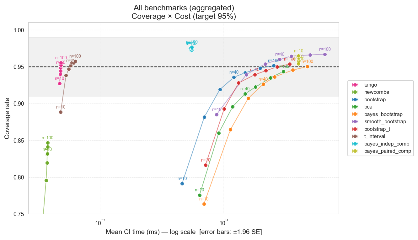
| Method | Coverage | Time (ms) | Width | Dev | Data types |
|---|---|---|---|---|---|
| Newcombe score interval | 0.816▼ | 0.037±0.000 | 0.2382 | -0.134 | Binary paired |
| BCa | 0.892▼ | 1.649±0.002 | 0.3272 | -0.058 | Any paired |
| Bayes bootstrap | 0.899▼ | 2.368±0.003 | 0.3214 | -0.051 | Any paired |
| Percentile bootstrap | 0.910▼ | 1.338±0.001 | 0.3242 | -0.040 | Any paired |
| Bootstrap-t | 0.918 | 1.892±0.002 | 0.3455 | -0.032 | Any paired |
| t_interval | 0.942 | 0.057±0.000 | 0.3593 | -0.008 | Any paired |
| Tango score interval ★ | 0.946 | 0.048±0.000 | 0.3111 | -0.004 | Binary paired |
| Smooth bootstrap (Gaussian KDE) | 0.948 | 3.242±0.004 | 0.3727 | -0.002 | Any paired |
| Bayesian paired comparison ★ | 0.958 | 4.076±0.000 | 0.3439 | +0.008 | Binary paired |
| Bayesian independent comparison | 0.975 | 0.551±0.000 | 0.3844 | +0.025 | Binary paired |
Coverage target is 0.95. ▼ marks under-target coverage. ★ marks preferred methods. Results are averaged across all benchmarks, model pairs, and sample sizes. Methods shown for all types (bootstrap, t-interval, etc.) are included for reference; in practice only binary-specific methods are applied to binary data.
Tango is still good, but it slightly under-covers at small N<50—so we can't entirely reproduce the strong result. Why?
Why does Tango under-cover at small N on real data?
When we looked more closely at which model pairs drive the under-coverage, two patterns emerge:
- Dominated pairs: one model scores near 0% on a benchmark while the other scores, say, 80%. The discordant pairs (inputs where the two models disagree) are too lopsided for Tango's score statistic to accumulate enough signal, and the CI ends up slightly too narrow.
- Jointly sparse pairs: both models score very low, e.g. both around 2%. Again, discordant pairs are too rare, and the CI ends up slightly too narrow.
These extreme situations are very common in our sample of OpenEval's benchmark, since we sample a diverse set of models at different parameter scales (e.g., a 1B model versus a 70B one), where the strong model dominates. Our synthetic simulation represented these extreme situations, but in the end, their results are averaged with more "well-behaved" pairs across a wide range of distributions.
In fact, we can see how it might be an artifact of the OpenEval sampling by running the same simulation on different LLM evals data—taking a single-run of the multi-run benchmark data we collected (explained below). When we do that, we see Tango again matches Bayesian paired:
CI Coverage vs. Computation Cost — Pairwise Binary (Real LLM Evals, Single-Run Subsample)
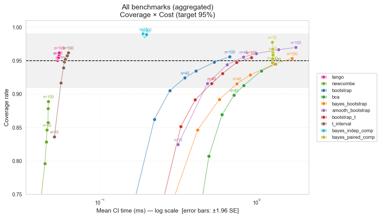
Figure: Coverage vs. computation cost for pairwise binary CI methods on real LLM eval data (single-run subsample of multi-run benchmarks), comparing Tango and Bayesian paired across sample sizes.
This pattern could also be an artifact of how the real-data simulation is constructed. Because we subsample from large benchmarks — and large benchmarks contain correlated items and difficulty clusters — a random draw of N = 20 items can easily land in a sparse or lopsided regime that would be unusual in a carefully curated, representative eval set. In a smaller, purpose-built evaluation that attempts reasonable coverage of difficulty, the dominance and sparsity problems would largely disappear.
Finally, the situations where Tango under-performs are also extreme cases where CIs don't tell us much —if one model completely dominates in performance (0% vs 80%), merely eyeballing mean differences may be enough. Similarly, if both models perform very poorly (2% vs 2%), statistics are similarly not that informative. So if a CI method is "slightly off", it may not be a big deal in practice.
That said, evalstats cannot base recommendations on "it's usually fine."
Since the failure mode exists and is observable on real benchmark data at small N, our recommendation changes:
- N < 50: use Bayesian paired with 10,000 resamples for binary pairwise CIs. It provides better small-sample coverage in the real-data regime, including the sparse/dominated cases where Tango struggles. We sacrifice speed considerably, but it's safer for extreme cases that may very well appear in practice on poorly constructed evaluation sets or "David vs. Goliath" scenarios.
- N ≥ 50: switch to Tango score interval. At this point Tango reaches its target coverage, is dramatically faster, produces tighter CIs than Bayesian paired, and sits closer to the nominal α level rather than over-covering. Critically, it also does not deteriorate at large N the way the Bayesian paired method does.
This threshold-based switch is what evalstats implements under method="auto"
for binary pairwise comparisons.
Multi-Run Coverage (Hierarchical Data)
Increasingly, it has become good practice to collect multiple "runs" per input, to account for the inherent stochasticity in LLM outputs. These multi-run scenarios introduce a second level of variance — run stochasticity within each input — that single-run methods ignore or may not even be able to handle. We ran a separate Monte Carlo simulation (200 MC reps; 10% of the single-run study) over the same distribution suite, sweeping both N (number of inputs) and f_run (runs per input), to compare "flat" methods that just use the mean of runs or take only the first run, against nested resampling methods. For a harder challenge that better matches real LLM eval data (where each "item" is really of different difficulty), run-level noise in these simulations is heteroscedastic: run noise variance differs across inputs.
The key finding is that taking the per-input mean across runs and running standard methods over those means performs reasonably well — Wilson, Tango, and NIG all achieve near-target coverage this way.
Input-level clustering is automatically absorbed when the mean is treated as a single observation, so these methods are not as badly hurt as truly flat approaches that treat every run as an independent data point.
However, tighter CI widths can be achieved with methods that explicitly account for within-item run variance: by decomposing total variance into a between-item term and a within-item Monte Carlo noise term (as in tango_multirun_mmnt and the nested resampling variants), the interval can be narrowed without sacrificing coverage.
The practical upshot is that running on means is a safe baseline, but if you have enough runs per input the multi-run-aware methods will give you meaningfully narrower intervals at no extra compute cost.
CI Coverage vs. Computation Cost — Point Estimates
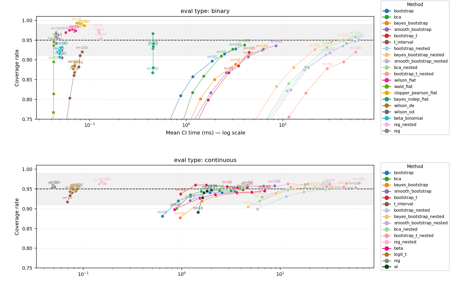
Figure: Coverage vs. computation cost for point-estimate (mean) CI methods in the multi-run setting, averaged across eval types, run-noise fractions, and sample sizes.
| Method | Coverage | Time (ms) | Width | Dev | Data types / Notes |
|---|---|---|---|---|---|
| bootstrap | 0.915 | 1.805±0.002 | 3.1739 | -0.035 | Any |
| bca | 0.921 | 2.272±0.002 | 3.1981 | -0.029 | Any |
| bayes_bootstrap | 0.912 | 3.230±0.004 | 3.1036 | -0.038 | Any |
| smooth_bootstrap | 0.935 | 4.375±0.005 | 3.6200 | -0.015 | Any |
| bootstrap_t | 0.924 | 2.552±0.003 | 3.6410 | -0.026 | Any |
| t_interval ★ | 0.924 | 0.080±0.000 | 3.5029 | -0.026 | Numeric only — near-target 0.95 for arbitrary-ranged data; appears here to under-cover due to subpar performance on binary 0/1 data |
| bootstrap_nested | 0.928 | 27.472±0.033 | 3.3464 | -0.022 | Any |
| bayes_bootstrap_nested | 0.935 | 21.073±0.026 | 3.4204 | -0.015 | Any |
| bca_nested | 0.936 | 28.137±0.034 | 3.3720 | -0.014 | Any |
| smooth_bootstrap_nested | 0.944 | 30.182±0.036 | 3.7742 | -0.006 | Any — best general-purpose nested method; near-exact coverage |
| bootstrap_t_nested | 0.928 | 28.214±0.034 | 3.6337 | -0.022 | Any |
| wilson_flat ★ | 0.974 | 0.066±0.000 | 0.2191 | +0.024 | Binary — simple, still performs well; takes mean of runs per item |
| wald_flat | 0.828▼ | 0.042±0.000 | 0.1838 | -0.122 | Binary only |
| clopper_pearson_flat | 0.989 | 0.083±0.000 | 0.2432 | +0.039 | Binary only |
| bayes_indep_flat | 0.920 | 0.454±0.002 | 0.2077 | -0.030 | Binary only |
| wilson_de | 0.881▼ | 0.069±0.000 | 0.1335 | -0.069 | Binary only |
| wilson_od | 0.918 | 0.051±0.000 | 0.1611 | -0.032 | Binary only |
| beta_binomial | 0.919 | 0.049±0.000 | 0.1606 | -0.031 | Binary only |
| nig_nested ★ | 0.966 | 0.144±0.000 | 0.1691 | +0.016 | Binary and continuous [0,1] — safer alternative to nig; most on-target method across synthetic and real data simulations |
| beta | 0.932 | 3.377±0.009 | 0.1443 | -0.018 | Continuous [0,1] |
| logit_t ★ | 0.949 | 0.079±0.000 | 0.1548 | -0.001 | Continuous [0,1] only — on-target and instant |
| nig ★ | 0.957 | 0.048±0.000 | 0.1606 | +0.007 | Binary and continuous [0,1] — for binary, takes mean of runs per item; slightly conservative, very fast |
| el | 0.933 | 1.729±0.003 | 0.1403 | -0.017 | Continuous [0,1] only |
Coverage target is 0.95. ▼ marks severe under-coverage. ★ marks preferred methods. 200 MC reps per condition. "Flat" methods treat multiple runs as independent observations and ignore run-level variance entirely. Nested methods resample inputs, then runs within inputs.
nig_nested work for binary data?
nig_nested is a hierarchical extension of the Normal-Inverse-Gamma (NIG) Bayesian credible
interval designed for multi-run data. The standard nig method places a NIG conjugate prior
on (μ, σ²) and returns an equal-tailed credible interval derived from the marginal
Student-t posterior for μ. The nested variant adapts this to an
(N, R) score matrix by explicitly decomposing variance into two levels: a
between-item component (variance of per-item means across inputs) and a
within-item component (average run-level variance divided by R). It then inflates the
sum-of-squares fed into the NIG update as
σ²eff = σ²item + σ²run / R,
so the posterior uncertainty automatically widens to reflect run noise — without needing any resampling.
What makes its binary performance surprising is that NIG is a Gaussian model, so there is no principled reason it should fit 0/1 data well. Yet it achieves 0.966 coverage, crucially remaining above 0.95 for all N, while remaining fast (0.14 ms). The likely explanation is that the hierarchical variance decomposition happens to produce a conservatively wide interval for binary data under the default weakly-informative prior, compensating for the model mismatch. This is somewhat accidental good behavior, as theoretically, a binomial model would be a more justified choice. It nevertheless earns the ★ as the most on-target method across both synthetic AND real-data simulations, outperforming or matching the other "more theoretically reasonable" Bayesian methods (beta-binomial, bayes_bootstrap_nested, and bayes_indep_flat) at lower cost. We can't argue with those results.
Multi-Run CI Method Performance for Pairwise Comparisons
CI Coverage vs. Computation Cost — Pairwise Comparisons
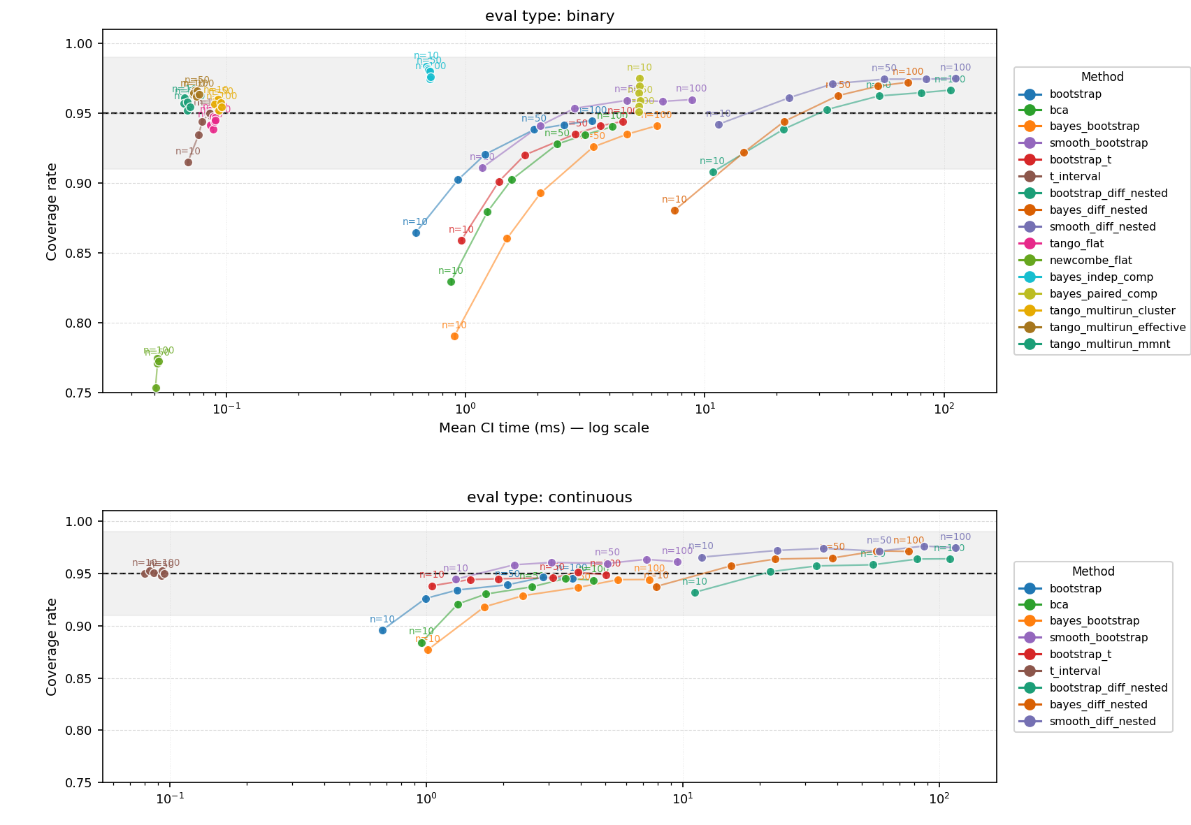
Figure: Coverage vs. computation cost for pairwise CI methods in the multi-run setting, averaged across eval types, run-noise fractions, and sample sizes.
| Method | Coverage | Time (ms) | Width | Dev | Data types / Notes |
|---|---|---|---|---|---|
| bootstrap | 0.927 | 1.932±0.002 | 1.9882 | -0.023 | Any paired |
| bca | 0.919 | 2.430±0.002 | 2.0047 | -0.031 | Any paired |
| bayes_bootstrap | 0.913 | 3.505±0.003 | 1.9516 | -0.037 | Any paired |
| smooth_bootstrap | 0.954 | 4.686±0.004 | 2.2674 | +0.004 | Any paired - under-covers for small N on binary data |
| bootstrap_t | 0.936 | 2.718±0.002 | 2.2593 | -0.014 | Any paired |
| t_interval ★ | 0.947 | 0.089±0.000 | 2.1927 | -0.003 | Numeric paired only — near-target and instant; aggregate under-coverage due to binary subpar performance |
| bootstrap_diff_nested | 0.955 | 51.815±0.049 | 2.2261 | +0.005 | Any paired — near-target but expensive |
| bayes_diff_nested | 0.956 | 35.782±0.033 | 2.3823 | +0.006 | Any paired — near-target; cheaper than bootstrap nested |
| smooth_diff_nested | 0.972 | 54.841±0.051 | 2.4805 | +0.022 | Any paired — safe and conservative even for small N on binary data; most expensive |
| tango_flat | 0.944 | 0.088±0.000 | 0.2775 | -0.006 | Binary only — fast flat binary pairwise method |
| newcombe_flat | 0.757▼ | 0.050±0.000 | 0.1874 | -0.193 | Binary only — severe under-coverage |
| bayes_indep_comp | 0.980 | 0.701±0.001 | 0.3486 | +0.030 | Binary only — over-covers; wide CIs |
| bayes_paired_comp | 0.962 | 5.333±0.003 | 0.3173 | +0.012 | Binary only — slightly over-covers |
| tango_multirun_cluster | 0.957 | 0.092±0.000 | 0.2174 | +0.007 | Binary only, multi-run — near-target and fast |
| tango_multirun_effective | 0.964 | 0.074±0.000 | 0.2256 | +0.014 | Binary only, multi-run — near-target and fast |
| tango_multirun_mmnt ★ | 0.957 | 0.068±0.000 | 0.2178 | +0.007 | Binary only, multi-run — best and cheapest; performs consistently in real data simulations |
Coverage target is 0.95. ▼ marks under-target coverage. ★ marks preferred methods. 200 MC reps per condition. Nested methods resample inputs then runs within inputs for each resample step, greatly increasing compute cost but properly accounting for run-level variance.
tango_multirun_mmnt: a GPT-5 invention?
tango_multirun_mmnt is the best-performing method—but, to the best of our knowledge,
it is an approach that did not exist in the
literature prior to this project. It emerged from a conversation with GPT-5, where we asked it
to extend the Tango paired-binary CI to the multi-run setting. GPT-5 proposed decomposing the
total variance of the per-item paired difference — computed as
delta_i = d10_i − d01_i (mean discordance rates across runs)
— into a between-item term and a within-item Monte Carlo noise term.
Crucially, it identified that naively using the observed item-level variance
Var(delta_i) would double-count the within-item run noise, and proposed subtracting
E[u_i − delta_i^2] / R (where
u_i = d10_i + d01_i is the discordance mass and R is
the number of runs) to recover the latent between-item variance. The resulting interval retains
Tango's score-shrinkage denominator and reduces exactly to the original Tango CI when
R = 1. Under simulation it achieves near-target coverage (0.957) while
being the fastest of the three multi-run Tango variants, making it the recommended default.
It is notable as an example of a novel statistical procedure generated by a language model
that holds up under both synthetic and real-data simulation.
Multi-Run Coverage with Real LLM Evals Data
Since we had run the other cases on real LLM eval data, we wanted to check if the multi-run results held up there as well. Unfortunately, we could not use OpenEvals (or any other public dataset) because they do not have multi-run data. (Only DOVE does, but they sample only 100 items per benchmark, which is too small for a coverage simulation.) Thus, we had to run benchmarks ourselves on a sample of models. For this test, we only ran benchmarks that produce binary scores, for two reasons: the Tango under-coverage problem was more pronounced there and we wanted to see if it held up on real data; and it is harder to find numeric score benchmarks.
We ran the following benchmarks and models using the Inspect AI benchmark harness and the OpenRouter API. This range of models was chosen as a good sample of model diversity in terms of provider and size:
- Benchmarks: MMLU, ARC, HellaSwag, GSM8K, WinoGrande, TruthfulQA, BoolQ, PIQA, BBQ
- Models: meta-llama/llama-3.1-8b-instruct, mistralai/ministral-8b-2512, google/gemma-3n-e4b-it, ibm-granite/granite-4.1-8b, qwen/qwen3.5-35b-a3b, openai/gpt-4o-mini
As you can see, the above results largely hold up on real data for the binary case. The one difference is that many methods are brought down a little, which is why we recommend NIG-nested here instead of NIG on means.
CI Coverage vs. Computation Cost — Point Estimates (Real LLM Evals)
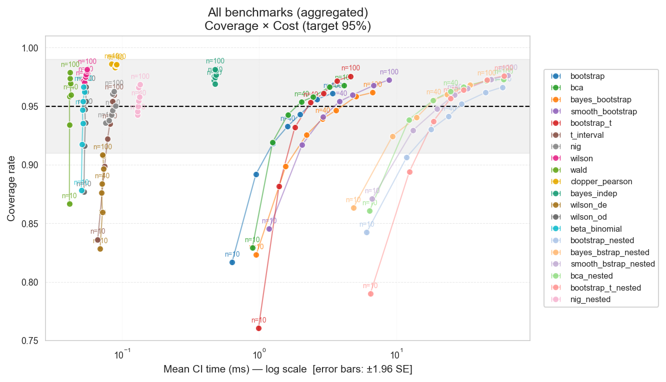
Figure: Coverage vs. computation cost for point-estimate CI methods in the multi-run setting, measured on real LLM eval data.
CI Coverage vs. Computation Cost — Pairwise Comparisons (Real LLM Evals)
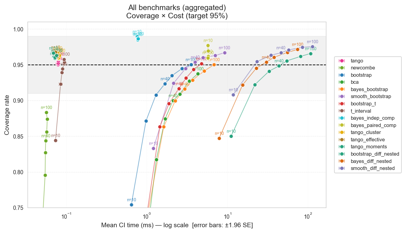
Figure: Coverage vs. computation cost for pairwise CI methods in the multi-run setting, measured on real LLM eval data.
Comparison with Bayesian Methods for Binary Scores
To address the ICML 2025 position paper arguing that practitioners should avoid CLT-style / frequentist
intervals for LLM evals in favor of Bayesian beta-posterior methods ("Don't Use the CLT in LLM Evals With Fewer Than a Few Hundred Datapoints"), we ensured the simulation included the exact Bayesian
methods the authors advocate, implemented using their bayes_evals library.
Our simulation results put some of their recommendations into question. For the binary scores 0/1, we find:
- Wilson score interval lands on target coverage (0.951 synthetic; 0.955 real data) at much cheaper computational cost, so the paper's preferred Bayesian alternative is not needed here.
- For the pairwise comparisons, the story is nuanced. In the synthetic simulation, Tango (0.955) matches Bayesian paired (0.958) in coverage while being nearly 100× faster. But on real LLM eval data — where dominated pairs and jointly-sparse model comparisons are common — Tango under-covers at N < 50, caused by extreme situations of sparse data regimes. Bayesian paired remains better in these small-sample setups. At N ≥ 50, Tango reaches target coverage, is dramatically faster, produces tighter intervals, and does not deteriorate at large N.
- In the new multi-run simulation, the NIG-nested variant achieves the highest point-estimate coverage overall (0.966), well above the authors' Bayesian independent samples method (0.920). NIG-nested is itself a Bayesian method — placing a Normal-Inverse-Gamma prior on (μ, σ²) and returning a marginal Student-t credible interval — but uses a Gaussian likelihood rather than a Binomial/Beta model. The result shows that the authors' specific Beta-posterior model is not uniquely suited to the hierarchical binary case; a different conjugate Gaussian model substantially outperforms it.
In the course of this analysis, we also uncovered a severe problem in the authors' library that makes it unsuitable for practical usage on benchmark data:
around N≈200+, the bayes_evals Bayesian
paired method begins to fail catastrophically with overconfident CIs that continue to decline as N increases.
(We ran additional simulations up to N=1000 confirming this pattern.
The reason why seems to be that the importance sampling procedure becomes unstable at larger N.)
Because of this failure mode, Bayesian paired is not recommended for N ≥ 100 — and it should never be used beyond N ≈ 200.
For small samples (N < 50), it retains a narrow use-case: real-data simulations show it handles dominated and jointly-sparse pairs better than Tango in that regime.
For larger samples, and as the default once N reaches 50, practitioners could switch to the Tango and Wilson intervals (and their multi-run analogues), which are fast, well-calibrated, and stable.
For multi-run data, which was not considered in the paper, practitioners should use NIG-nested for point estimates and Tango's multi-run variant for pairwise comparisons.
Is BCa bootstrap a good method for estimating CIs?
If you chat with an LLM, it might start to go off about how BCa is the gold standard. Don't listen to it. BCa is actually one of the worst methods in most of our simulations. We aren't the only skeptics, either. One simulation study found:
This is consistent with our own simulation results on both synthetic and real LLM eval data.
Simultaneous Confidence Intervals for Multiple Comparisons
When comparing multiple prompts or models, it is common to run multiple pairwise comparisons. In these cases, controlling the family-wise error rate (FWER) is essential to avoid spurious findings. The max-T resampling procedure is a well-established method in genomics and neuroscience for constructing simultaneous confidence intervals (CIs) that jointly cover all comparisons, rather than treating each CI in isolation (basically, it widens the CIs to ensure the alpha level is maintained across all comparisons). It also has very few assumptions, allowing for robust inference even when candidates are correlated. Despite its power and flexibility, max-T is virtually unknown in LLM evaluation and ML contexts.
The max-T procedure works by resampling the data (e.g., via bootstrap), computing the test statistic (such as the difference in means) for all pairs in each resample, and then recording the maximum absolute value of the test statistics across all comparisons for each resample. The distribution of these maxima is then used to set CI bounds that guarantee the desired coverage simultaneously for all comparisons, not just marginally. This approach is less conservative than Bonferroni correction, yet provides strong control over false positives.
evalstats uses the max-T procedure by default whenever you output multiple pairwise comparisons with bootstrapped CIs. This ensures that the reported intervals account for the increased uncertainty from making many comparisons at once. For consistency, evalstats also applies the max-T correction to p-values when users request them, so that both CIs and p-values are corrected in the same principled way.
The max-T method is recommended by Rink & Brannath, 2025, a recent ML paper on multiple comparisons correction when comparing many candidate models that may be correlated. For more foundational background, see the Methods Used in evalstats and Statistical Pitfalls in ML sections of the Resources page.
Which p-value Method Works Best?
We also ran another Monte Carlo simulation study to compare p-value methods for pairwise
testing across LLM eval data types and sample sizes, implemented in
simulations/sim_compare_pvalues.py. The criterion here is Type I error
control under the null (target: α = 0.05) plus consistency across
data distributions and N.
Wilcoxon Signed Ranks is our recommended default for pairwise
comparisons for those adopting a NHST framework. In this simulation, it is slightly conservative, consistently
performant across sample sizes, data types, and distributions, and does not show pathological
behavior where Type I error is inflated above the nominal threshold
(α = 0.05). Wilcoxon is a non-parametric test that
makes fewer assumptions about the data distribution, which likely contributes
to its robustness in this context. It is also widely implemented, well-understood,
and computationally efficient, making it a practical choice for developers.
That said, the Sign Test is also a reasonable choice for safety-critical settings where false positives are especially costly, because it is much more conservative than Wilcoxon.
For comparing 3+ models/prompts, we recommend the Friedman test as the default, with Wilcoxon signed ranks as the post-hoc pairwise test. Friedman is a non-parametric test for comparing more than two related samples, it doesn't assume normality, and it's robust to homoscedasticity (variance of residuals). Friedman tests are already used in some ML contexts for comparing models, as advocated by Demsar (2006). Note that evalstats does not output Friedman by default, since it does not foreground a NHST-style analysis pipeline, but it is available as an option for users who want to use it.
For multiple comparisons correction,
we recommend the Benjamini-Hochberg procedure (correction="fdr_bh")
to those in lower-stakes contexts, as it which performed comparably to other methods in our simulation,
but had the greatest power among methods that maintained Type I error control.
In extremely safety-critical contexts, the Bonferroni-Holm correction (correction="holm")
is more appropriate for its strong control over false positives, albeit at the cost of increased false negatives.
We ran simulations to provide guidance on which p-value method is most reliable for LLM evals, for those who want to use them, but we do not recommend relying on p-values. Null-hypothesis significance testing (NHST) should not be the primary basis for eval decisions. A p-value is only a compatibility check against a null model; it does not tell you the magnitude, direction, or practical importance of an effect.
If you report p-values at all, always report them alongside effect sizes and confidence intervals. In practice, prefer effect sizes and CIs as the main evidence, and use p-values as secondary context. Prefer alpha thresholds that are more conservative than 0.05, if you use them at all (e.g., 0.001).